
This tutorial will cover basic techniques for financial data analysis. Specifically, we will use the pandas library to import stock data and manipulate the data to identify an investment thesis. This tutorial is targeted at complete beginners, keep in mind that because of their simplicity these techniques won’t make you any money; they are designed to inspire you to investigate further.
Step 1: Installing prerequisites
Assuming you’re running the latest version of Python 3, we will need to install a couple of basic packages:
pip3 install numpypip3 install matplotlibpip3 install pandaspip3 install pandas-datareaderpip3 install beautifulsoup4pip3 install sklearnpip3 install quandl
If you would like to learn more about Matplotlib visit our tutorial on the subject here. Likewise we have a great tutorial on data analysis with pandas.
Step 2: Imports
To begin with we will need to do some imports of modules we will be using throughout the tutorial.
import datetime as dtimport matplotlib.pyplot as pltfrom matplotlib import styleimport pandas as pdimport pandas_datareader.data as web
We'll be using date-time to work with dates, matplotlib will allow us to create graphs and pandas should let us manipulate data.
Step 3: Setup
Now lets prepare some variables and imports for manipulation later on.
style.use('ggplot')start = dt.datetime(2018, 1, 1)end = dt.datetime.now()
qkey = 'YOUR API KEY HERE'
df = web.DataReader('WIKI/GOOGL', 'quandl', start, end, access_key=qkey)
First things first our graphs should look good, style.use allows us to do this, ggplot is typically the better looking of the themes.
Next we create start and end variables, so we can easily call the same date-range in multiple contexts.
In order to get data from the Quandl API you would have to register on their website and get the API key first. You can register here, once registered confirm your email address and get your API key from 'account settings' and place it inside the qkey variable.
Finally, we use pandas DataReader to request Stockmarket data from the Quandl API, in this case we are requesting Google trading data since the beginning of the year (start) until present (end).
After running the above we should call the first 10 rows of the dataframe to confirm that everything is working correctly. So lets run:
df.head()
This should output table with the first 10 rows of information.
Step 4: Looking at the data
If you're new to the stockmarket and trading, this data may not be the easiest to understand. Below is a quick primer on what sort of inforamtin we're getting from the dataframe
- Open - The price of a share at the time when the stockmarket opens for morning trading.
- High - The highest value recorded during the trading day.
- Low - The lowest value recorded during the trading day.
- Close - The final price when the Stockmarket was closed.
- Volume - The number of shares traded for the day
- Adj. Open / Adj. High / Adj. Low / Adj. Close - Unlike the normal open, close, low, high, values the adjusted versions attempt to account for a stock split/splits in the ticker's history. Some companies can choose to do a stock split where they say every share is not worth two shares, splitting the value in half. Adjusted values are helpful as they account for stock splits, providing a price relative to the split. This is why you should mostly use adjusted values.
Step 5: Graphing the data
In order to start graphing the data all we need to do is run:
df.plot()plt.show()
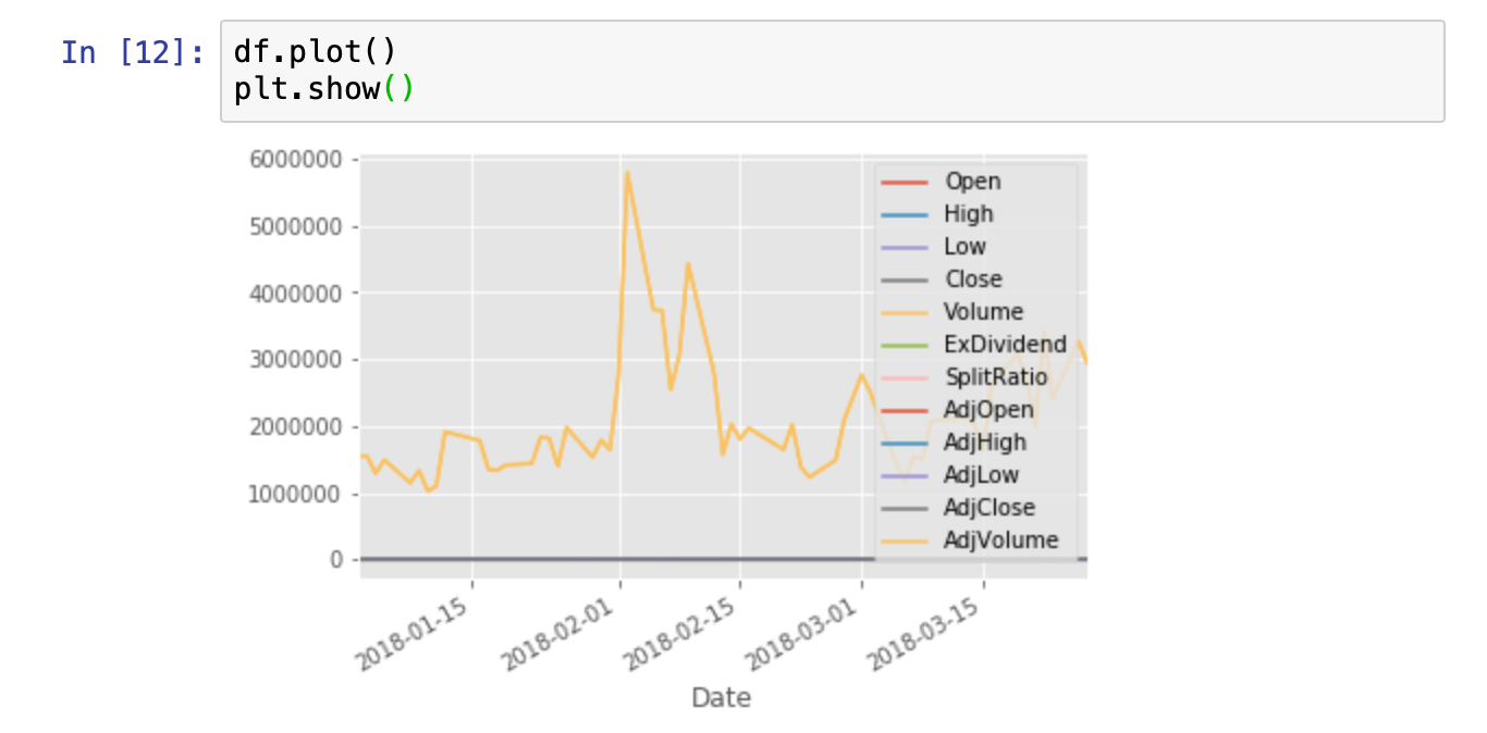
Unfortunately, since the Volume data is at a much greater scale than the other columns all we see is the volume graph.
But we can reference specific columns in the data frame by running:
df['AdjClose'].plot()plt.show()
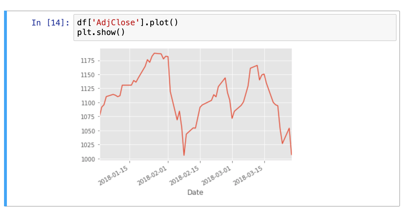
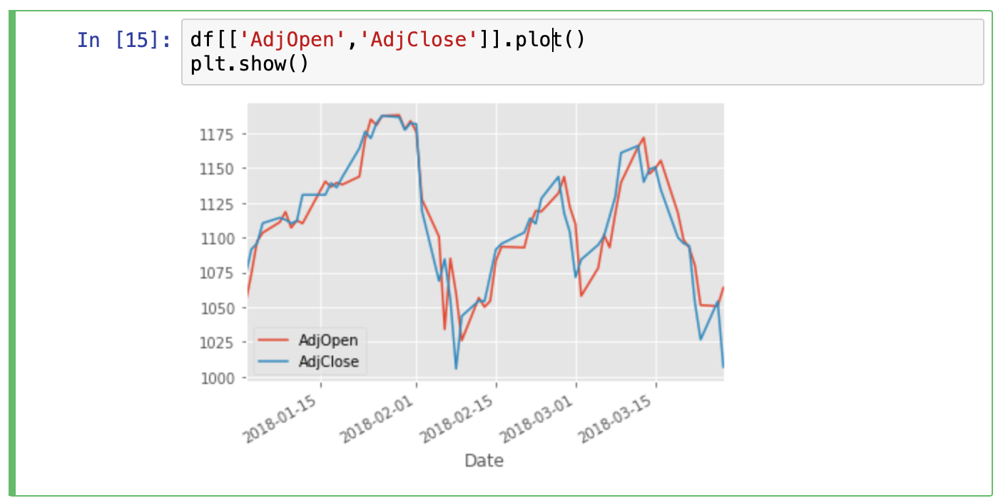
Now the result is much clearer and no key is displayed since we are only viewing one column. We can also graph multiple columns simultaneously:
df[['AdjOpen','AdjClose']].plot()
plt.show()
Conclusion
Thats it for the first part of our tutorial on Financial data with Python. Naturally, there is much more we could do here, but this should give you a solid foundation for the next tutorials in our series. Let me know what you thought of the tutorial in the comments and if you have any requests.
Appendix #1: Saving to CSV
We can also easily save the data to a csv, so as not to have to keep making API requests.
df.to_csv('google.csv')
Now instead of getting the data from an API every time, we could just use the .csv file instead.
df = pd.read_csv('google.csv', parse_dates=True, index_col=0)