
The Pandas library is the key library for Data Science and Analytics and a good place to start for beginners. Often called the "Excel & SQL of Python, on steroids" because of the powerful tools Pandas gives you for editing two-dimensional data tables in Python and manipulating large datasets with ease. In this short introduction to Pandas, I’ll show you the most frequently used functions for Analysts and Data Scientists. Since this is the first article on Pandas on this site we'll start from the basics.
Installation
Firstly you will need to install Pandas onto your machine/ environment. In this guide we will be using Jupyter Notebooks as this is the most common setup for Data Analysts. (Python version 3.7 the latest version available at the moment of writing) and because Jupyter Notebooks is excellent for beginners just getting started with Data Analysis.
Pandas install with Anaconda
The easiest way to install Jupyter Notebooks and Pandas set-up is to using the Anaconda distribution - a cross-platform distribution for data analysis and scientific computing. You can download the Windows, OS X and Linux versions of Anaconda. Anaconda Python distribution provides Jupiter Notebooks, together with a list of common Python packages which includes Pandas. After running the installer, you will have access to Pandas and the rest of the SciPy stack without needing to install anything else.
If for some reason your Anaconda set-up does not have Pandas you can add it manually with the following command (terminal MacOS or linux)
conda install pandas
Pandas install from PyPI
Pandas can also be installed directly on your machine via pip from PyPI.
pip install pandas
pip install numpy
While NumPy does not require any other packages, but Pandas does, so make sure you get them all. The installation order is not important.
A full Pandas installation guide from Pandas creators can be found here.
Start your Jupyter Notebook and test Paunads install by running the following .
import pandas as pd
import numpy as np
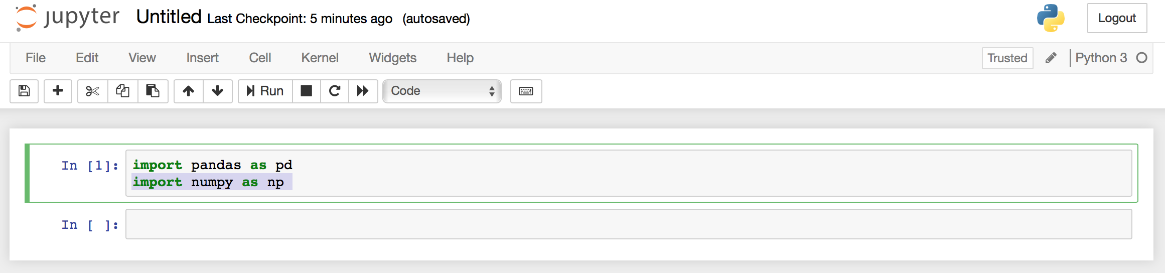
If you are not getting an error message everything was installed correctly.
Pandas Data Structures: DataFrame and Series
Pandas has two types of data structures : Series and DataFrames.
Series
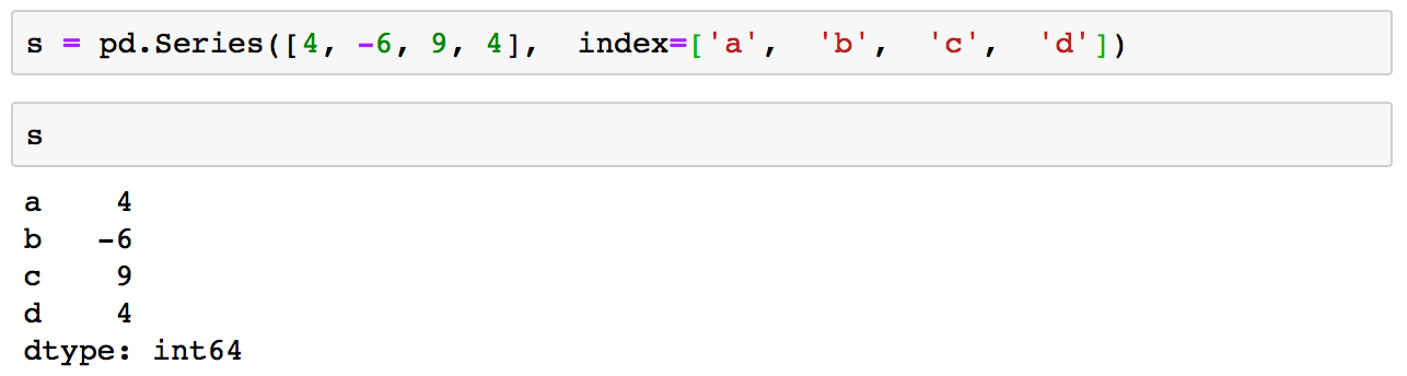
Pandas Series is a one dimentional data structure (labeled array) capable of holding any data type.
You can create a series with:
s = pd.Series([4, -6, 9, 4], index=['a', 'b', 'c', 'd'])
DataFrames
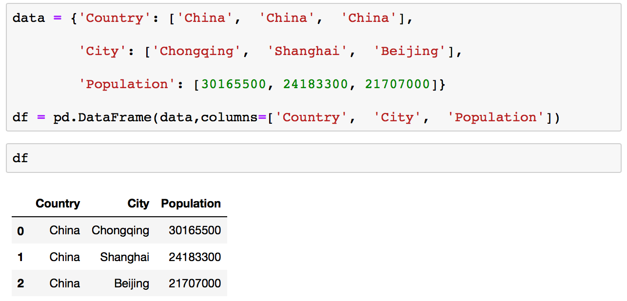
A Pandas DataFrame is a two dimensional data structure (a table with rows and columns).
You can create DataFrames manually in Pandas or by importing data from files.
The simplest way to create a DataFrame is by typing the data into Python manually, which obviously only works for tiny datasets.
data = {'Country': ['China', 'China', 'China'], 'City': ['Chongqing', 'Shanghai', 'Beijing'], 'Population': [30165500, 24183300, 21707000]}
df = pd.DataFrame(data,columns=['Country', 'City', 'Population'])
Importing and Saving Data with Pandas
What’s great about Pandas is that its designed to work with data in common formats like a CSV, JSON, TXT, TSV file, or a SQL database and creates a Python object with rows and columns is called a data-frame. Data-frames in Pandas look very similar to typical spreadsheet. In comparison to working with lists and/or dictionaries through for loops or list comprehension data-frames are so much easier to work.
Read and Write to CSV
You can import data from a csv file using the .read_csv() command. Note that df is a standard name for a data-frame, but you can call you data-frame anything you like.
df = pd.read_csv('file_name.csv')
If you want to save your data-frame from Pandas into a CSV file use the to_csv command.
df.to_csv('myDataFrame.csv')
Read and Write to Excel
Excel is one of the most common data formats especially when dealing with small datasets. You can read an excel file the same way you read a csv:
df = pd.read_excel('file_name.xlsx')
You can save your data-frame using bellow.
df.to_excel('file_name.xlsx')
To specify the sheet name, just add the sheet name parameter:
df.to_excel('file_name.xlsx', sheet_name = 'sheet1')
Read multiple sheets from the same excel file
If you need to read multiple worksheets of the same workbook try pd.ExcelFile:
xlsx = pd.ExcelFile('excel_file.xls')df = pd.read_excel(xlsx, 'Sheet1')
Read from Clipboard
You can even create a DataFrame from your clipboard as long as your Jupyter notebook is run on your machine and not in the cloud with pandas.read_clipboard.
df = pd.read_clipboard
Viewing Data in Pandas
Now that you know how to load data it is logical to ask how you can view it. In Jupyter notebooks you can just type name of your DataFrame and Python will show it to you. This is a convenient way to preview your loaded data, but this is not the same as opening file in Excel. Pandas by default only shows 100 rows and 20 columns.
Show your DataFrame (here DataFrame was named df):
df
If you load a wide data dataframe you’ll notice that Pandas displays only 20 columns, and only 60 or so rows, truncating the middle section. If the default behaviour does not satisfy you, just edit the defaults using set_option() for Pandas displays :
pd.set_option('display.max_rows', 500)
pd.set_option('display.max_columns', 500)
pd.set_option('display.width', 1000)
Checking the number of rows and the number of columns in a DataFrame
Scrolling through a big DataFrame to check if all rows and columns are loaded can be tidious. So instead of inspecting line by line just run the .shape command.
df.shape
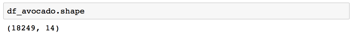
In my example DataFrame df_avocado contains 18,249 rows, each with 14 columns as shown above in the output of .shape.
You can also check number of dimensions in your DataFrame with .ndim command. If your DataFrame is created by loading a csv file you should expect two dimensions.
df.ndim

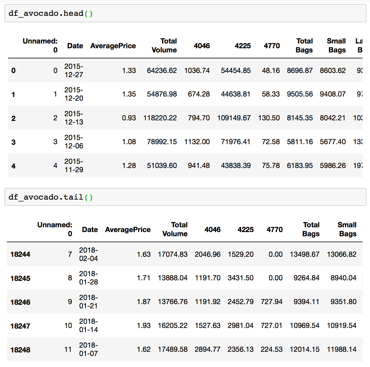
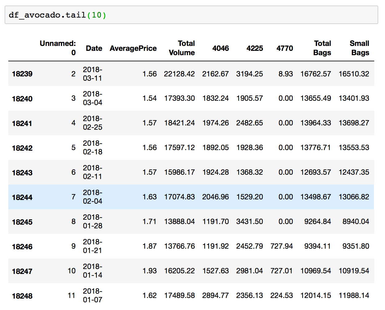
Display first rows or bottom rows with head() and tail()
The .head() function in Pandas, by default, displays the top 5 rows of data in the DataFrame. While function .tail() does the opposite, it gives you the last 5 rows. You can pass any number of rows into the commands for display.
df.head() or df.head(100)
df.tail() or df.head(50)
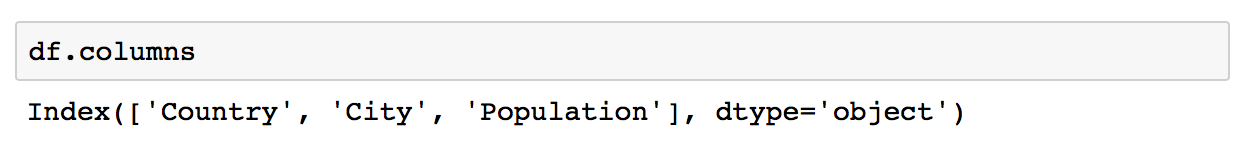
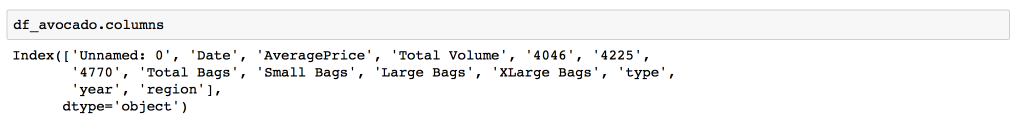
Displaying columns in you DataFrame
If you have a wide DataFrame not all columns will fit on the screen, so you will be scrolling alot. Doing this can be tricky when you need to copy a column name, or if you already run multiple commands and getting back to the DataFrame means scrolling in your notebook or running another .head() command. You can save yourself some time by running the .columns command instead, this will print out all columns in the DataFrame.
df.columns
Data types of columns in a DataFrame
Many DataFrames have mixed data types, where some columns are numbers, some are strings, and some are dates etc. While, CSV files do not contain information on what data types are contained in each column Pandas infers the data types when loading the data. So if a column contains only numbers, pandas will set that column’s data type to numeric: integer or float.
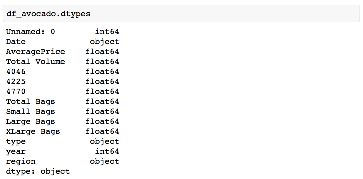
You can see the types assigned to each column with the .dtypes :
df.dtypes
If you want to see more information about your DataFrame in one place you can use .info() :
df.info()
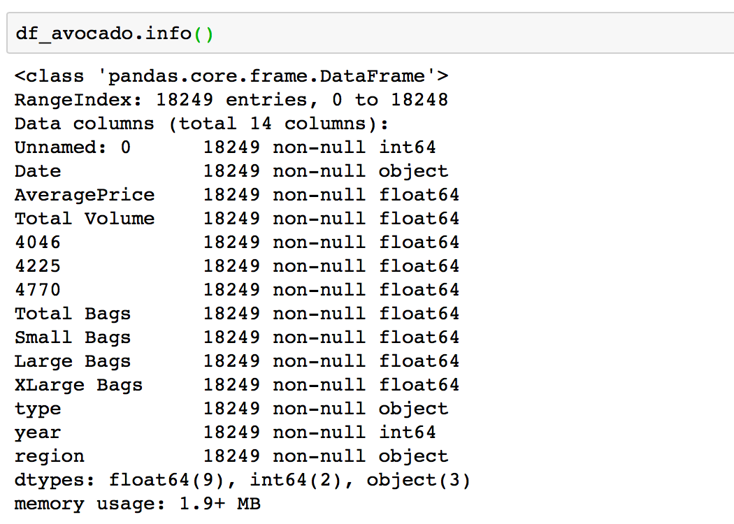
.info() will print a concise summary of a DataFrame.
This method prints information about a DataFrame including the index dtype and column dtypes, non-null values and memory usage.
Count non-null values in the DataFrame
In real worls spreadsheets quite often contain missing or null data. This can present challenges when analysing data, so it is important to check you imported DataFrame for null values. This can easily be done with .count():
df.count()
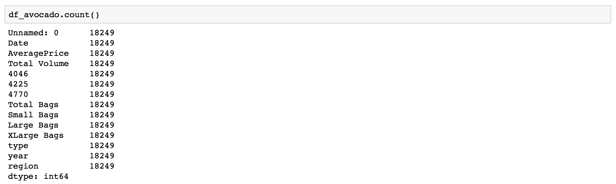
In my exsample all values are present, but this is a rear case of clean data. Avocado data came from Kaggel and was created with data analysis in mind.
Selecting and Indexing data
Pandas Indexing using [ ], .loc[], .iloc[ ]
There are plenty of ways to pull the columns and rows from a DataFrame. There are some indexing method in Pandas which help in getting the right element of data from a DataFrame. These indexing methods may look very similar but behave very differently. Pandas support four types of Multi-axes indexing they are:
- Dataframe.[ ] - This function also known as indexing operator.
- Dataframe.loc[ ]: - This function is used for labels.
- Dataframe.iloc[ ]: - This function is used for positions or integer based.
- Dataframe.ix[ ]: - Starting in 0.20.0, the
.ixindexer is deprecated, in favor of the more strict.ilocand.locindexers.
All together they are called the indexers. These are the standart ways to index data. These are four function which help in getting the elements, rows, and columns from a DataFrame.
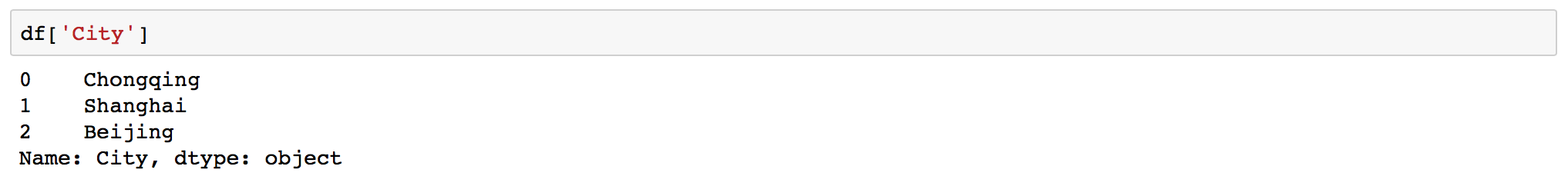
Selecting a column using indexing operator []
Selecting a column is easy all you need to do is type ['your column name'] after the DataFrame:
df['column']
Selecting row by index
df.loc[index]
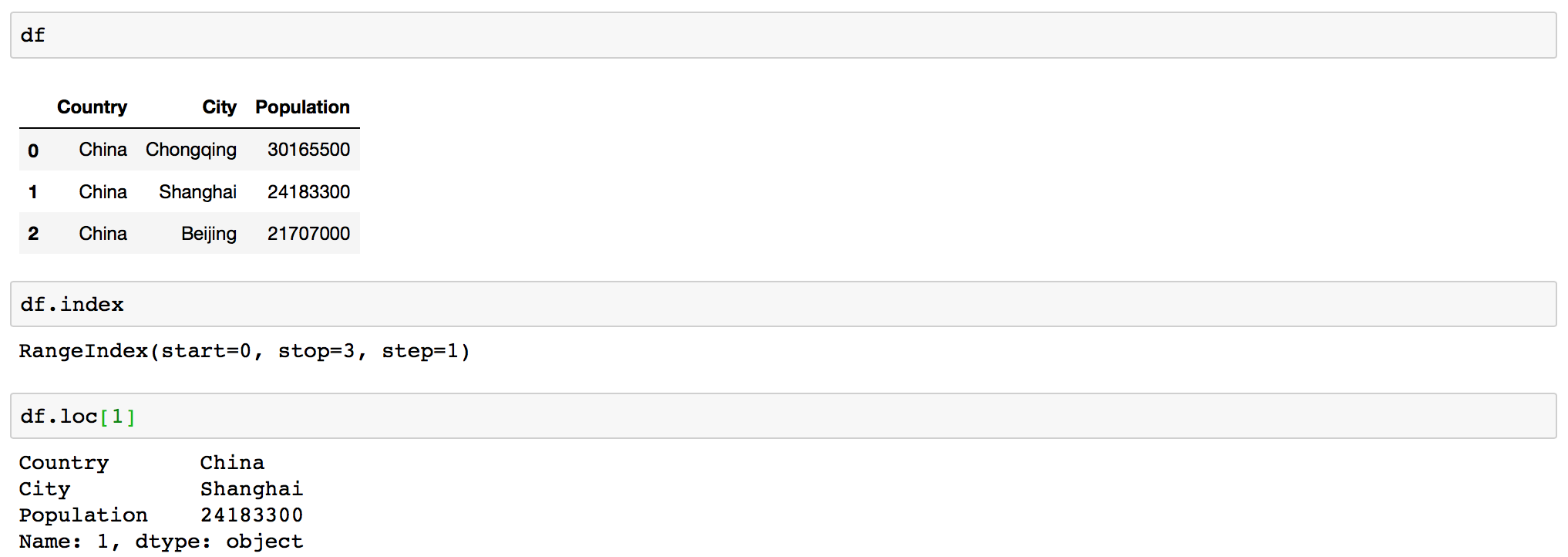
Do not forget that python starts indexing from 0. So if you want second row you need to ask for index 1.
Selecting in Pandas based on values in a column
To select rows whose column value equals a scalar, some_value, use ==:
Note that = sign in python taken for assignment, so if want to specify equality you need to use == instead.
df.loc[df['column'] == some_value]To select rows whose column value is in an iterable, some_values, use isin:
df.loc[df['column'].isin(some_values)]Combine multiple conditions with &:
df.loc[(df['column'] >= A) & (df['column_name'] <= B)]Note the parentheses. Due to Python's operator precedence rules, &binds more tightly than <=and >=. Thus, the parentheses in the last example are necessary.
To select rows whose column value does not equalsome_value, use !=:
df.loc[df['column'] != some_value]isinreturns a boolean Series, so to select rows whose value is not in some_values, negate the boolean Series using ~:
df.loc[~df['column_name'].isin(some_values)]Summarising Data
Getting basic stats for your DataFrame with .describe()
Now that you inspected your DataFrame and know how to select specific data from a DataFrame it is time to get some basic statistics about it. When you run .describe() on the whole dataframe it prints out statistics for numeric columns by default.
df.describe()
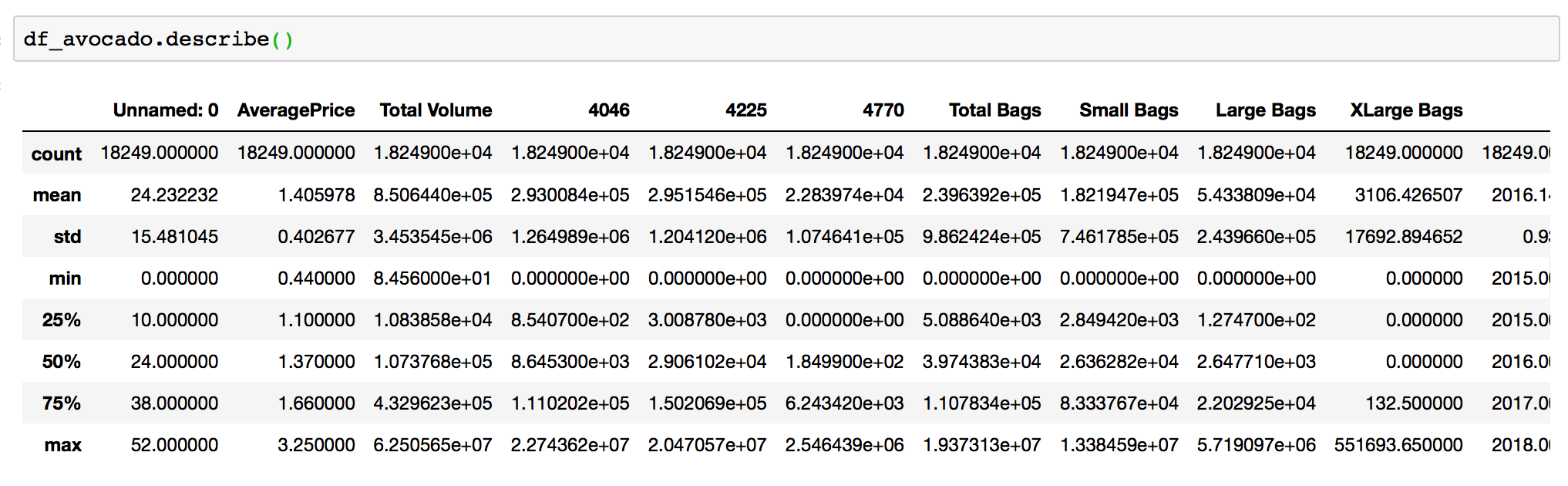
For numeric columns describe() return such basic statistics as: the value count, mean, standard deviation, minimum, maximum, and 25th, 50th, and 75th quantiles for the data in a column.
Meanwhile, for string columns describe() returns the value count, the number of unique entries, the most frequently occurring value (‘top’), and the number of times the top value occurs (‘freq’).
Counts of unique values with value_counts()
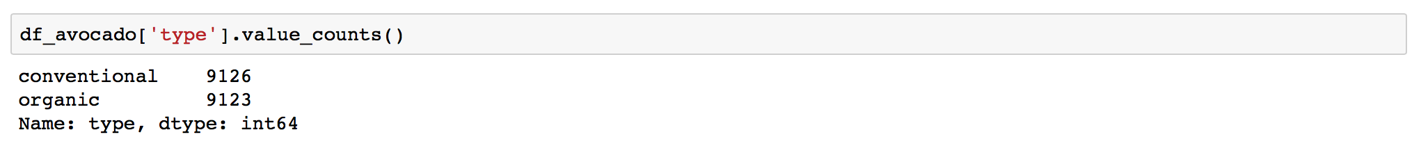
You canget a count of number of rows with each unique value of variable using .value_counts() :
df['column'].value_counts()
It doesn't usually make sense to perform value_counts on a DataFrame. Instead this command should be used on a specific column. Running this command without specifying a column will result in an error: AttributeError: 'DataFrame' object has no attribute 'value_counts'.
This command will return an object that will be in descending order so that the first element is the most frequently-occurring element. Excludes NA values by default.
Counting unique values with .nunique().
You can request a count of distinct values in a column with .nunique() :
df['column'].nunique()

Uniques are returned in order of appearance. Hash table-based unique, therefore does NOT sort.
Listing unique values with .unique()
If you want to see unique values in the column you can use .unique() for this:
df['column'].unique()

This will output an array with unique values. If their are too many unique values in the column some of them will not be displayed in the Jupyter notebooks by default.
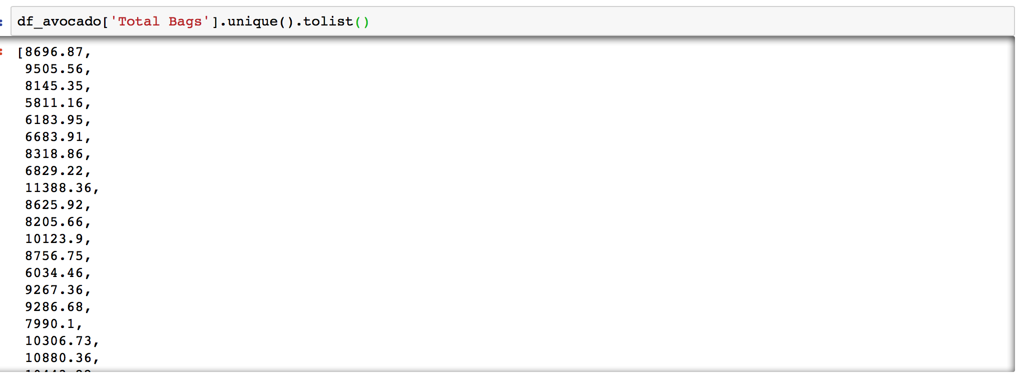
If you want a list of unique values it is better to run .unique().tolist():
df['column'].unique().tolist()
List of Summary functions
Pandas provides a large set of summary functions that produce single values for each of the groups. When applied to a DataFrame, the result is returned as a pandas Series for each column. Examples:
.sum() - Sum values of each object.
.median() - Median value of each object.
.quantile([0.25,0.75]) - Quantiles of each object.
.min() -Minimum value in each object.
.max() - Maximum value in each object.
.mean() - Mean value of each object.
.var() - Variance of each object.
.std() - Standard deviation of each object.
.mad() - Mean absolute deviation from mean value.
.skew() - Sample skewness (3rd moment) of values.
.kurt() - Sample kurtosis (4th moment) of values.
.cumsum() - Cumulative sum of values.
.cumprod() - Cumulative product of values.
.pct_change() - Computes percent changes.
Manipulating data
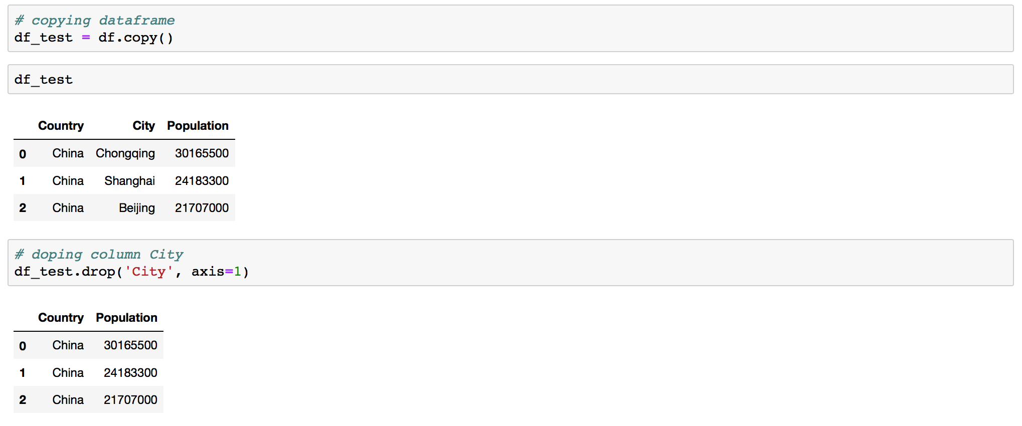
Dropping column from DataFrame in Pandas
You can drop column with .drop() :
df.drop('column', axis =1)
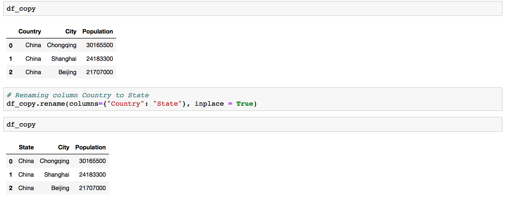
Renaming column in Pandas
Renaming a column in Pandas can be asily achived by using the DataFrame .rename() function. The rename function is easy to use, and quite flexible.
df.rename(columns={"old_column_name": "new_column_name"}, inplace =True
Handling Missing Data
When you encounter missing data you have a number of options for handling missing data: Filtering out missing data or Filling in missing data.
Filtering out missing is done with .dropna()
df.dropna()
Filling in missing data is done with .fillna(value)
df.fillna(value)
Conclusion
Python Pandas are great for data munging and preparation and so is a great way to start your data analysis journey. Pandas helps fill this gap, enabling you to carry out your entire data analysis workflow in Python without having to switch to difrent tools and learn other languages.
However if you want to do sophisticated modeling it most likely would not be enough. Pandas does not implement significant modeling functionality outside of linear and panel regression; for this, look to such Python libraries as statsmodels and scikit-learn.